
Fractals, those telescoping self-similar filigree meshes that marry mathematics and art, have become so mainstream, that they are even mentioned in the theme song of Disney’s 2013 mega-hit, Frozen.
My power flurries through the air into the ground
Let it Go, by Idina Menzel (Frozen, Disney 2013)
My soul is spiraling in frozen fractals all around
And one thought crystallizes like an icy blast
I’m never going back, the past is in the past
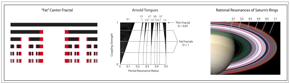
But not all fractals are cut from the same cloth. Some are thin and some are fat. The thin ones are the ones we know best, adorning the cover of books and magazines. But the fat ones may be more common and may play important roles, such as in the stability of celestial orbits in a many-planet neighborhood, or in the stability and structure of Saturn’s rings.
To get a handle on fat fractals, we will start with a familiar thin one, the zero-measure Cantor set.
The Zero-Measure Cantor Set
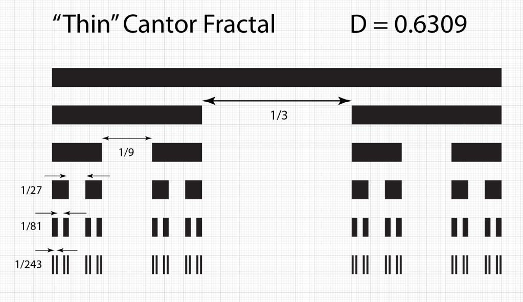
The famous one-third Cantor set is often the first fractal that you encounter in any introduction to fractals. (See my blog on a short history of fractals.) It lives on a one-dimensional line, and its iterative construction is intuitive and simple.
Start with a long thin bar of unit length. Then remove the middle third, leaving the endpoints. This leaves two identical bars of one-third length each. Next, remove the open middle third of each of these, again leaving the endpoints, leaving behind section pairs of one-nineth length. Then repeat ad infinitum. The points of the line that remain–all those segment endpoints–are the Cantor set.
The Cantor set has a fractal dimension that is easily calculated by noting that at each stage there are two elements (N = 2) that divided by three in size (b = 3). The fractal dimension is then

It is easy to prove that the collection of points of the Cantor set have no length because all of the length was removed.
For instance, at the first level, one third of the length was removed. At the second level, two segments of one-nineth length were removed. At the third level, four segments of one-twenty-sevength length were removed, and so on. Mathematically, this is
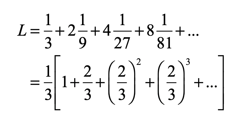
The infinite series in the brackets is a binomial series with the simple solution
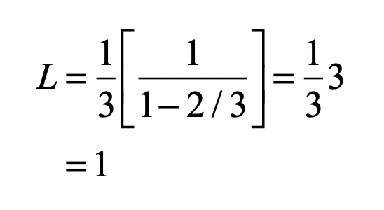
Therefore, all the length has been removed, and none is left to the Cantor set, which is simply a collection of all the endpoints of all the segments that were removed.
The Cantor set is said to have a Lebesgue measure of zero. It behaves as a dust of isolated points.
A close relative of the Cantor set is the Sierpinski Carpet which is the two-dimensional analog. It begins with a square of unit side, then the middle third is removed (one nineth of the three-by-three array of square of one-third side), and so on.
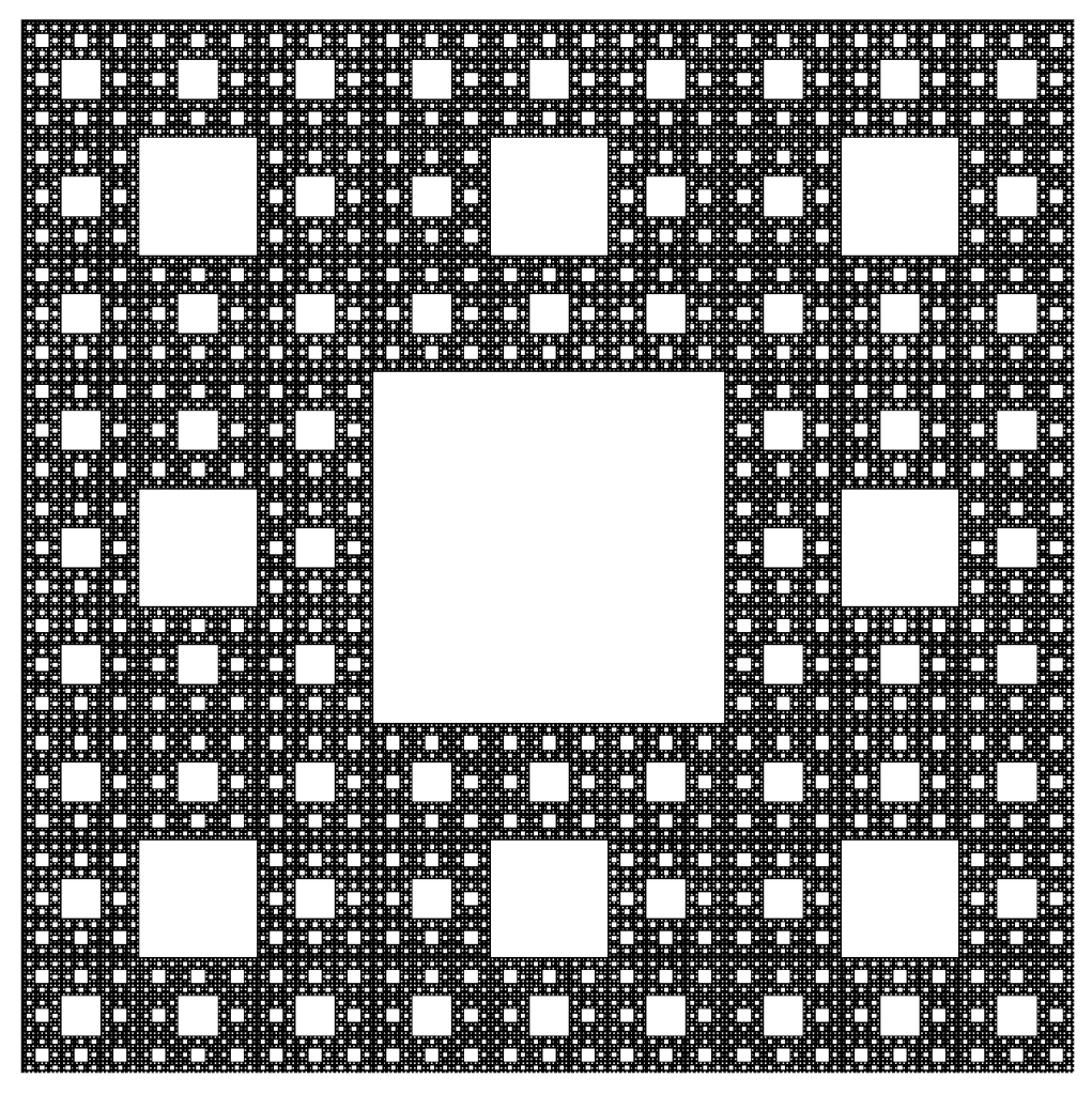
The resulting Sierpinski Carpet has zero Lebesgue measure, just like the Cantor dust, because all the area has been removed.
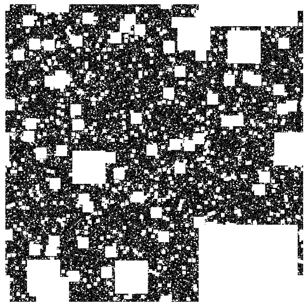
There are also random Sierpinski Carpets as the sub-squares are removed from random locations.
These fractals are “thin”, so-called because they are dusts with zero measure.
But the construction was constructed just so, such that the sum over all the removed sub-lengths summed to unity. What if less material had been taken at each step? What happens?
Fat Fractals
Instead of taking one-third of the original length, take instead one-fourth. But keep the one-third scaling level-to-level, as for the original Cantor Set.

The total length removed is
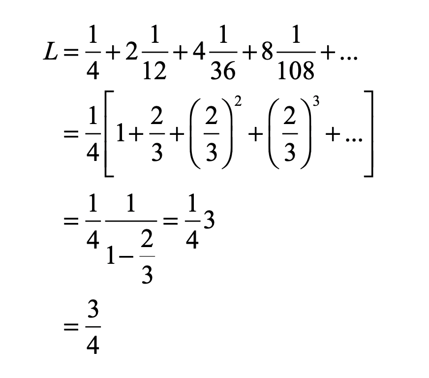
Therefore, three fourths of the length was removed, leaving behind one fourth of the material. Not only that, but the material left behind is contiguous—solid lengths. At each level, a little bit of the original bar remains, and still remains at the next level and the next. Therefore, it is said to have a Lebesgue measure of unity. This construction leads to a “fat” fractal.
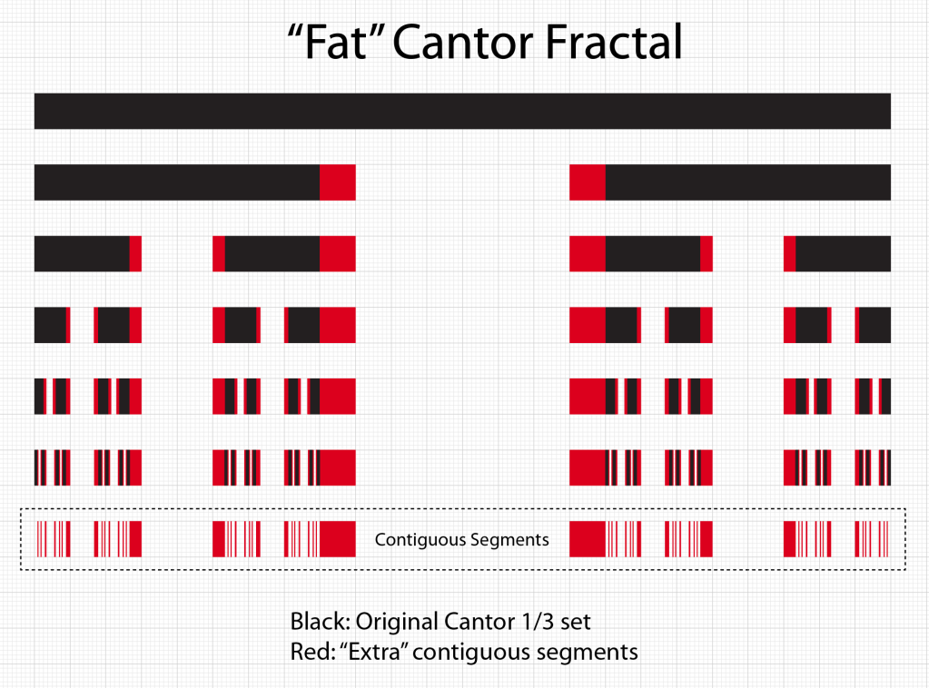
Looking at Fig. 5, it is clear that the original Cantor dust is still present as the black segments interspersed among the red parts of the bar that are contiguous. But when two sets are added that have different “dimensions”, then the combined set has the larger dimension of the two, which is one-dimensional in this case. The fat Cantor set is one dimensional. One can still study its scaling properties, leading to another type of dimension known as an exterior measure [1], but where do such fat fractals occur? Why do they matter?
One answer is that they lie within the oddly named “Arnold Tongues” that arise in the study of synchronization and resonance connected to the stability of the solar system and the safety of its inhabitants.
Arnold Tongues
The study of synchronization explores and explains how two or more non-identical oscillators can lock themselves onto a common shared oscillation. For two systems to synchronize requires autonomous oscillators (like planetary orbits) with a period-dependent interaction (like gravity). Such interactions are “resonant” when the periods of the two orbits are integer ratios of each other, like 1:2 or 2:3. Such resonances ensure that there is a periodic forcing caused by the interaction that is some multiple of the orbital period. Think of tapping a rotating bicycle wheel twice per cycle or three times per cycle. Even if you are a little off in your timing, you can lock the tire rotation rate to a multiple of your tapping frequency. But if you are too far off on your timing, then the wheel will turn independently of your tapping.
Because rational ratios of integers are plentiful, there can be an intricate interplay between locked frequencies and unlocked frequencies. When the rotation rate is close to a resonance, then the wheel can frequency-lock to the tapping. Plotting the regions where the wheel synchronizes or not as a function of the frequency ratio and also as a function of the strength of the tapping leads to one of the iconic images of nonlinear dynamics: the Arnold tongue diagram.
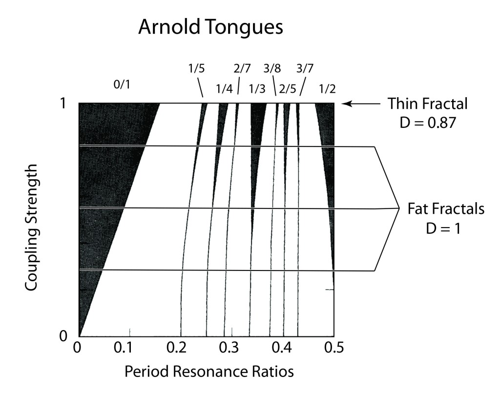
The Arnold tongues in Fig. 6 are the frequency locked regions (black) as a function of frequency ratio and coupling strength g. The black regions correspond to rational ratios of frequencies. For g = 1, the set outside frequency-locked regions (the white regions are “ergodic”, as the phase of the oscillator runs through all possible values) is a thin fractal with D = 0.87. For g < 1, the sets outside the frequency locked regions along a horizontal (at constant g) are fat fractals with topological dimension D = 1. For fat fractals, the fractal dimension is irrelevant, and another scaling exponent takes on central importance.
The Lebesgue measure μ of the ergodic regions (the regions that are not frequency locked) is a function of the coupling strength varying from μ = 1 at g = 0 to μ = 0 at g = 1. When the pattern is coarse-grained at a scale ε, then the scaling of a fat fractal is

where β is the scaling exponent that characterizes the fat fractal.
From numerical studies [2] there is strong evidence that β = 2/3 for the fat fractals of Arnold Tongues.
The Rings of Saturn
Arnold Tongues arise in KAM theory on the stability of the solar system (See my blog on KAM and how number theory protects us from the chaos of the cosmos). Fortunately, Jupiter is the largest perturbation to Earth’s orbit, but its influence, while non-zero, is not enough to seriously affect our stability. However, there is a part of the solar system where rational resonances are not only large but dominant: Saturn’s rings.
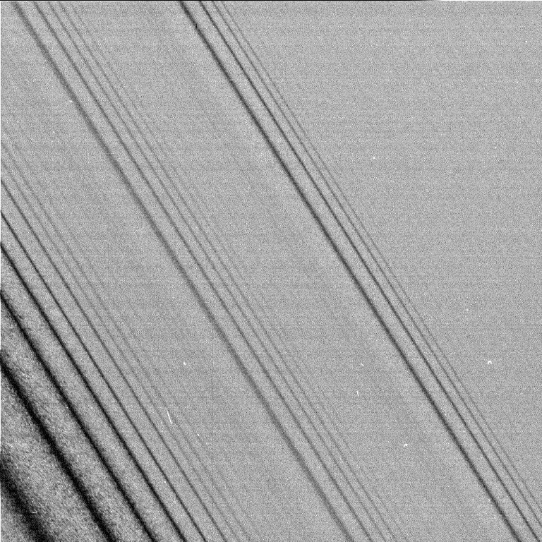
Saturn’s rings are composed of dust and ice particles that orbit Saturn with a range of orbital periods. When one of these periods is a rational fraction of the orbital period of a moon, then a resonance condition is satisfied. Saturn has many moons, producing highly corrugated patterns in Saturn’s rings at rational resonances of the periods.
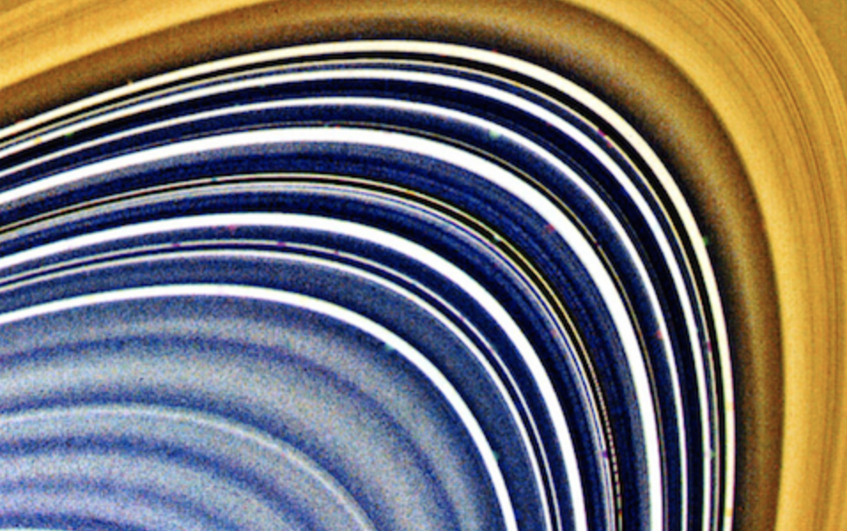
The moons Janus and Epithemeus share an orbit around Saturn in a rare 1:1 resonance in which they swap positions every four years. Their combined gravity excites density ripples in Saturn’s rings, photographed by the Cassini spacecraft and shown in Fig. 8.
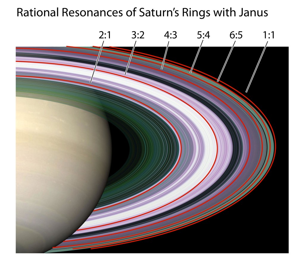
One Canadian astronomy group converted the resonances of the moon Janus into a musical score to commenorate Cassini’s final dive into the planet Saturn in 2017. The Janus resonances are shown in Fig. 9 against the pattern of Saturn’s rings.
Saturn’s rings, orbital resonances, Arnold tongues and fat fractals provide a beautiful example of the power of dynamics to create structure, and the primary role that structure plays in deciphering the physics of complex systems.
References:
[1] C. Grebogi, S. W. McDonald, E. Ott, and J. A. Yorke, “EXTERIOR DIMENSION OF FAT FRACTALS,” Physics Letters A 110, 1-4 (1985).
[2] R. E. Ecke, J. D. Farmer, and D. K. Umberger, “Scaling of the Arnold tongues,” Nonlinearity 2, 175-196 (1989).
