For many people, the reproduction of recorded sounds takes place in a conceptual black box: sound goes in, and sound comes out, and it’s stored up in things called “records” in between, but the process itself is all very mysterious.  Because of that, the claim that we can play back pictures of sound waves (which seem to be very different things from “records”) is often met with incredulity.  The technique I’ll be describing here “defies belief,” according to Gizmodo.

But really there’s nothing magical or even particularly surprising about the fact that we can turn pictures of audio waveforms into sound.  After all, if you look closely at the groove of a 78 rpm record or a mono LP, you’ll see that it’s nothing more than an incised waveform coiled into a long spiral.  Because the waveform is incised in depth, it can physically guide a stylus back and forth through its undulations as the disc revolves, which gives us a convenient means of transducing them into an audible sound wave.  But the information is all there in the two-dimensional path of the waveform itself.  Barring issues of resolution, there’s no more information in a 78 rpm record or a mono LP than there would be in a picture of the same waveform printed on a piece of paper.  If we want to listen to a waveform inscribed two-dimensionally on a piece of paper, the challenge we face is the practical one of transferring that information into a playable form.  Of course, it’s not incised sufficiently in depth to guide a stylus on a turntable.  But we can scan the picture of the waveform, convert the digital image data into a digital sound file, and then play the sound file.  That’s what I’m going to describe how to do.

One possible name for this practice would be paleokymophony (“old-wave-sounding”).  It’s one of two basic approaches I’ve been using to educe historical sonic inscriptions as sound—that is, to “play” them, to actualize them for sensory perception from a latent or potential state.  The other is paleospectrophony, which I’ve written about here.  The distinction between the two methods is that paleospectrophony interprets data as a graph of frequency as a function of time, whereas paleokymophony (or whatever else we choose to call it) interprets data as a graph of amplitude as a function of time.  These are the two methods I used to produce the audio for Pictures of Sound, published in 2012 by Dust-to-Digital.

[Update, November 20, 2016: since publishing this blog post, I’ve written some code of my own that accomplishes the same thing as the method described below, but better and more simply—check it out.]

1. Isolate the trace as a white line on a black background.

If the trace starts out as a dark trace on a light background, invert it so that it’s a light trace on a dark background.  It’s also generally useful to increase the contrast—often multiple times at the maximum setting in Photoshop—and then to fill the background in with black using the paintbucket tool, always being careful not to lose any detail of the wave shape itself.

2. Adjust the waveform image so that its center or “zero point” coincides with a straight line running from left to right.

If the waveform is coiled into a spiral, as in the case of a gramophone disc, then we need to “de-spiral” it.  In Photoshop use Filter > Distort > Polar Coordinates, with the “Polar to Rectangular” radio button selected.  This is a memory-intensive transform, and you’ll need a lot of RAM to carry it out on larger images; I splurged on an Asus G74S specifically for this purpose.  It’s also unavailable for images over 30,000 pixels in any direction.  Be careful to center the spiral as exactly as you can, bearing in mind that the outermost revolution of the spiral isn’t equidistant from the center (because its midpoint moves gradually outward).  An imperfectly centered spiral yields “wavy” rows after the transformation.  I never seem to be able to get the centering exactly right myself, but I try to get pretty close.  Getting it wrong is equivalent to playing a gramophone disc on a turntable slightly off center.

A waveform often creeps gradually up the page, as illustrated in exaggerated form below.  We want to isolate it into the narrowest rectangular strip of image we can.  In Photoshop, we can use Edit > Transform > Skew to reorient it; be sure to drag the handle at the midpoint of the side of the selection box rather than one of the corners.  You can do this with a single trace or with a large number of parallel traces all at once (such as the above example shown after de-spiraling).

If the amplitude axis is itself skewed at an angle rather than oriented straight up and down relative to the time axis, we can also use the “skew” function to adjust its azimuth as shown here (top is “before,” bottom is “after”):

3. If you’re working with a number of sequential segments of a trace, join as many of them together into a single very long image file as feasible.

Starting with the de-spiraled version of the gramophone disc shown above, for example, we would need to cut out the individual rows or revolutions one by one and join them end to end.

The main challenge here lies in lining up the splices correctly, both vertically and horizontally.  If you’re dealing with a trace with an irregular or compromised seam between rotations or revolutions, it’s useful to make one layer transparent so that you can slide the images over the top of one another to find the overlap that best preserves the cyclicality of the waveform.  Here’s an example of such a join from one of Édouard-Léon Scott de Martinville’ phonautograms (#47, “Et Incarnatus Est”), with vocal trace below and simultaneous tuning-fork trace above:

Images in Photoshop are limited to 300,000 pixels in any direction, so longer recordings will need to be divided into multiple 300,000-pixel segments.  In that case, be sure to leave some overlap between segments so that when it comes time to splice together the resulting WAV files you can choose a conspicuous and convenient landmark they both share in common to serve as the transition point.

4. If there are any breaks in the trace, repair them manually.

This process can be more or less time-consuming and subjective depending on how much of the trace is missing.  Here’s a relatively straightforward example from a photographic record of the phrase “How do you do?” as captured in 1878 by Eli Whitney Blake, Jr., showing breaks in the trace drawn in by hand with a pencil tool:

Now imagine what would be involved in doing the same thing for the vocal trace in the phonautogram of “Et Incarnatus Est” shown above, and you’ll get a sense for how labor-intensive this step can be.  If there’s any visual noise remaining in the background at this point, such as blotches or specks, that will need to be cleaned up as well.  Overall, the process closely resembles the retouching of historical photographs.

5. Create two copies of the waveform image, one with the area above the trace filled in white (using the paintbucket tool), and the other with the area below the trace filled in white.

The goal here is to convert amplitude values—that is, how far “up” or “down” the trace is at each successive point in time—into different amounts of whiteness or brightness.  This strategy pertains only to “wavy line” representations of sound waves; if you have the good fortune to be working with an oscillographic image that already varies in brightness, such as an optical film sound track, then you can skip steps 4, 5, and 7.  Here are a few other examples of cases where that observation applies: from top to bottom, manometric flames photographed by Edward L. Nichols and Ernest Merritt (1898), a vertically modulated phonograph cylinder as read by IRENE, and an illustrative plate from Leonhard Euler’s Tentamen novae theoriae musicae (1739):

Some of the other processing steps may still be necessary in these instances, such as azimuth correction (in the top example), separation into rows (in the middle example), and inversion to black on white (in the bottom example).  By analogy with the traditional distinction between vertically and laterally modulated recordings, I refer to this alternative approach as vertical eduction, as opposed to the lateral eduction that takes place with wavy lines.

6. Run the images through software designed to convert optical sound track images into WAV files.

The software I’ve been using for this purpose is Andrew Jaremko’s ImageToSound, a piece of freeware designed to convert images into sound as though they were optical film sound tracks (where the modulation of the audio signal is tied to how much light passes through a translucent strip that varies either in width or opacity).   It’s getting increasingly difficult to find online, but it can still be downloaded here as of November 2014.  This program converts each successive pixel column in an image file into one audio sample, the value of which is calculated as the sum of the luminance of all pixels in the column—in the scenario I’m describing, this equals the amount of white in each successive pixel column, which corresponds in turn to the vertical displacement of the original trace.  In effect, we’re measuring distances from the edges of the image to the edges of the trace, like this:

ImageToSound is limited to processing 24-bit BMPs, so it’s necessary to convert image files into that format if they aren’t already in it.  The program is also restricted to outputting an 8-bit WAV, although the user can choose the sample rate (I generally go with 44.1 kHz).  A few other quirks about it are worth noting:

• It won’t run in Windows 7, except in Windows 98 compatibility mode, and in that mode I’ve found that it can’t handle some of the larger files that it was able to accommodate in earlier versions of Windows.  I maintain a desktop computer running Windows 98 to handle those cases.
• It removes some DC offset, which might be advantageous from the standpoint of experimental sound art, but which isn’t desirable for my purposes because it compromises the accuracy of the eduction.  I sometimes mitigate the effect by running the images through both forwards and backwards (i.e., horizontally flipped) and combining the results (after reversing the backwards file); this works pretty well.  But in doing that, I run into another problem: for some reason, the output WAV files don’t start and stop exactly with the first and last pixels of the images, so the “forward” and “backward” versions don’t line up exactly.  My strategy for dealing with this other problem has been to insert a single column of white pixels at the far left of the “forward” image before flipping it to create the “backward” image; this creates a single-sample tick in both resulting WAV files that I can use as a common reference point for lining them up with sample-perfect precision.  In fact, it’s advantageous to insert several of these single-pixel columns, since I’ve occasionally found one of them inexplicably cropped out of one of the output WAVs.
• Sometimes ImageToSound returns a WAV file that lacks the usual resolution: the single-sample tick vanishes and finer details go missing throughout.  I don’t know what causes the problem, but changing the width of the image to a rounder number (by expanding the canvas size) seems to fix it.

I’m grateful that ImageToSound exists, but I’d like to see someone design a piece of software that doesn’t have these shortcomings.  AEO-Light seems to have promise as an alternative tool for accomplishing the same thing better and more flexibly, but I haven’t yet succeeded in getting it to work.

Because the approach I’ve described doesn’t involve following or tracking the trace itself, it can accommodate distortions that technically violate the logic of the time-amplitude graph, such as “loopback,” where the trace seems to move backwards relative to the time axis.  It can’t actually correct such distortions; that would require some kind of geometrical manipulation that has yet to be accomplished.  But it can at least educe them in a consistent way that also yields accurate results from undistorted traces.

7. Now it’s just a matter of carrying out some basic audio editing processes.  Combine the two output WAV files into a stereo file, placing the top-filled version in the left channel and the bottom-filled version in the right channel.  Invert the left channel.  Then sum the two channels to mono.

8. Adjust the playback speed.

If you’ve converted the image into audio at a sample rate of 44,100 kHz, then each second of audio initially corresponds to a width of 44,100 pixels in the input image.  If you know the original recording speed, you can adjust the playback speed accordingly.  Let’s say that your original source image was a spiral recorded at a constant angular velocity of 50 revolutions per minute, and that—after de-spiraling—each revolution occupies 30,000 pixels.  30,000 pixels per revolution × 50 revolutions per minute = 1,500,000 pixels per minute; divided by 60, that comes out to 25,000 pixels per second.  Take the duration of the output file at 44,100 pixels per second, multiply it by 1.764 (44,100 / 25,000) to calculate the target duration, and then resample the file to that target duration.  On the other hand, if you don’t know the original recording speed, you can still try to adjust the playback speed by ear.

That’s assuming the recording was made at a constant speed.  If you’re dealing with a recording that was made at an irregular speed, then you may want to try to correct the irregularity.  For recordings made with a tuning-fork reference trace, like this—

—combine the WAVs of the “main” trace and the tuning-fork trace into a stereo file.  Then select each group of five cycles in the tuning-fork trace and manually set it to a constant duration:

If you know the frequency of the tuning fork in Hertz, then divide five by that number to get the target duration for each group of five cycles.  Alternatively, if you don’t know the frequency, find the longest duration occupied by five cycles, set everything to that duration, and adjust the speed by ear once the fluctuations have been factored out.  Be sure always to select the same point in the tuning-fork cycle for your starting and ending points.  You can choose to work with some number of cycles other than five, of course, but I’ve found that five-cycle groups tend to work pretty well.

If a recording was made at an irregular speed without a reference trace, you can’t correct the speed fluctuations objectively, but you may still be able to restore something close to the original speed based on inferences about the source material (e.g., a scale played on a cornet) or manual cranking patterns (which tend to have some degree of regularity to them).  Not much has yet been done along these lines, but it’s a field ripe for exploration.

9. Enjoy the results!  Here are a few choice examples.

A paper print of an experimental gramophone recording made by inventor Emile Berliner on November 11, 1889, located by Stephan Puille in a scrapbook at the Library of Congress.  In the excerpt given here, Berliner counts from one to twenty in English, laughs heartily, and sings “Reiters Morgengesang”—to the best of my knowledge, this is the earliest known recording of singing in the German language.

---

A phonautogram of “Au Clair de la Lune” as sung by inventor Édouard-Léon Scott de Martinville on April 9, 1860, scanned and made audible by the First Sounds initiative.  This is the world’s oldest known recording of the human voice with audibly recognizable subject matter (i.e., if you know the song, you’ll recognize it from the playback).  I’ve presented three successive versions to illustrate the steps that went into processing it: (1) vocal trace and tuning-fork trace in stereo without speed correction; (2) vocal trace and tuning-fork trace in stereo with speed correction; (3) vocal trace in mono with speed correction.

I created the sound file of “Au Clair de la Lune” provided here back in 2011 using the image-to-sound processing technique outlined above.  However, the version originally we released to the public in 2008 had instead been converted into audio by “virtual stylus” software devised at Lawrence Berkeley National Laboratory as part of the IRENE project, which centers on using optical scanning technology to extract data from analog grooved media for playback.  For comparison, here’s a graphic that shows a snippet of the 2011 eduction (top), the original scanned trace (middle), and the 2008 eduction (bottom):

The 2011 eduction follows the trace more accurately, but that’s due mainly to intensive manual cleanup of the source image.  In the 2008 eduction, you can see points at which visual noise confused the Berkeley algorithm; detecting the pattern in such cases may require the intervention of a human being, something like a CAPTCHA.  I should mention that the image-to-sound processing techniques I’ve outlined in this blog post can also be applied successfully to the raw optical output of IRENE.  To illustrate the point, here’s a brief audio clip based on data extracted by IRENE at NEDCC from a phonograph cylinder of the “Anvil Chorus,” converted into sound using my methods rather than the IRENE team’s own PRISM software:

---

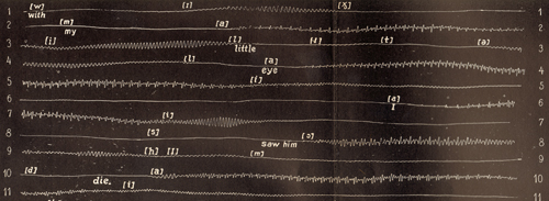Waveform of the spoken phrase “With my little eye, I saw him die,” transferred by Edward Wheeler Scripture from a commercial gramophone disc onto paper and published in Researches in Experimental Phonetics: The Study of Speech Curves (Washington DC: Carnegie Institution of Washington, 1906).  This trace forms part of the cover art for Pictures of Sound.

---

Two waveforms of the spoken phrase “How do you do?” as recorded photographically by Eli Whitney Blake, Jr.: an original print found in the Alexander Graham Bell papers at the Library of Congress.  An edited version of the bottom trace was published in the American Journal of Science for July 1878 and was mentioned as already published in the Boston Daily Advertiser of July 9, 1878.  Hence the recording itself must have been made long enough before July 9, 1878, for it to have been written up, reviewed, accepted, engraved, printed, and distributed by that date.  The big question is whether this process took more or less than seventeen days.  After all, if the recording predates June 22, 1878—the date of a St. Louis tinfoil recording that was played back optically in 2012, revealing a couple nursery rhymes—then that would make it the oldest specimen of recognizably recorded spoken English yet recovered.

---

And finally, here’s a phonautogram of the famous Alexander Graham Bell saying “ah” on January 28, 1875!

 

I threw that one in just to show that not every waveform ends up yielding compelling audio content—my First Sounds colleagues and I refer to results like these as “thwips and farts.”  They may not sound like much, but they’re still conceptually cool and can be harnessed for creative purposes, as with this little musical composition I threw together back in 2008 based on a phonautographic “thwip” from 1857:

Now it’s your turn.  Go find a picture of a waveform and see what you can do!